When speeding makes sense — Fast, consistent, durable and scalable streaming data with Pravega

By Raúl Gracia on Posted on October 1, 2020 in Performance

Introduction

Streaming systems continuously ingest and process data from a variety of data sources. They build on append-only data structures to enable efficient write and read access, targeting low-latency end-to-end. As more of the data sources in applications are machines, the expected volume of continuously generated data has been growing and is expected to grow further [1][2]. Such growth puts pressure on streaming systems to handle machine-generated workloads not only with low latency, but also with high throughput to accommodate high volumes of data.

Pravega (“good speed” in Sanskrit) is an open-source storage system for streams that we have built from the ground up to ingest data from continuous data sources and meet the stringent requirements of such streaming workloads. It provides the ability to store an unbounded amount of data per stream using tiered storage while being elastic, durable and consistent. Both the write and read paths of Pravega have been designed to provide low latency along with high throughput for event streams in addition to features such as long-term retention and stream scaling. This post is a performance evaluation of Pravega focusing on the ability of reading and writing.

To contrast with different design choices, we additionally show results from other systems: Apache Kafka and Apache Pulsar. Initially qualified as messaging systems, both Pulsar and Kafka make a conscious effort to become more like a storage system; they have recently added features like tiered storage. These systems have made fundamentally different design choices, however, leading to different behavior and performance characteristics that we explore in this post.

The main aspects covered in this post and the highlights of our results are the following:

Overall ingestion performance. A Pravega writer produces over 1 million events per second for small events (100 bytes) and sustains 350MB/s throughput for large events (10,000 bytes), both with single-digit millisecond latency (at the 95th percentile).
Durability. Pravega always makes the data durable on acknowledgment. The write throughput of Kafka is at least 40% less compared to Pravega for a single-segment stream, independent of flushing on every message or not. For a 16-segment stream, the Pravega writer provides comparable throughput to the Kafka writer flushing on every message, but Pravega write latency is lower (i.e., single-digit millisecond vs. 1+ seconds for Kafka).
Dynamically adjusting batches. Pravega does not require a complex configuration for client batching. The Pulsar client can achieve either low latency or high throughput, but not both. For Kafka, configuring large batches is detrimental for throughput when the application uses routing keys (throughput is 80% lower for a 16-segment stream). In both cases, forcing the user to statically configure batching is undesirable.
Behavior in the presence of large events for throughput-oriented workloads. Pravega obtains up to 350MB/s for a 16-segment stream with 10kB events. The throughput is 40% higher than the one of Pulsar and comparable to the throughput of Kafka (about 6% difference). However, the latency in the case of Kafka is over 800ms while the one of Pravega is in single-digit milliseconds.
End-to-end latency. When tailing a stream, the Pravega reader also provides single-digit millisecond latency end-to-end while serving data at high throughput. It provides a higher throughput (roughly 80% more) for a single-segment stream when compared to Kafka. For Pulsar, adding partitions and readers leads to lower performance (single-partition case achieves 3.6x the throughput of the 16-segment case).
Use of routing keys. Pravega does not present any significant performance difference when using or omitting routing keys. For moderate/high throughput rates, Kafka and Pulsar show over 2x end-to-end latency when using routing keys and, specifically for Kafka, a maximum read throughput that is over 37% lower.
Tiered storage for catch-up and historical reads. Pravega can catch up with 100GB of historical data dynamically while ingesting 100MB per second of new data. Pulsar with tiering enabled was not able to catch up for the same scenario, inducing a backlog that grows without bounds.
Performance with auto-scaling. Auto-scaling is a unique feature of Pravega. Scaling up a stream provides higher ingestion performance. We show that scaling up a stream using a constant ingestion rate of 100MB/s causes write latency to drop.

Except when we show time series, we plot latency along with throughput. It is a problem we commonly find across blog posts; they plot either latency or throughput, whereas both are jointly relevant for streaming workloads. For example, the maximum throughput for a given configuration might look very good while the latency is of the order of hundreds of milliseconds to a few seconds. We plot latency-throughput graphs to avoid misleading conclusions. We additionally provide tables with the data points used to complement the plots. The tables give more data than the plots (e.g., different percentile ranks) for completeness.

Background

Pravega is a complex system, and we encourage the reader to investigate further our documentation, including previous blog posts. Here, we provide a very brief summary of the write and read paths, along with some key points of Kafka and Pulsar.

The Pravega write path

Pravega has different APIs for adding data to a stream. In this section, we primarily focus on the event stream API.

The event stream writer writes events to a stream. A stream can have parallel segments that can change dynamically according to an auto-scaling policy. When an application provides routing keys, the client uses them to map events to segments. If the routing key is omitted when writing an event, then the client selects a segment randomly.

The client opportunistically batches event data, and writes such batches to a segment. The client controls when to open new batches and close them, but the data for a batch accumulates on the server. The component in Pravega managing segments is called the segment store. The segment store receives such requests to write to a segment, and both add the data to a cache and appends it to a durable log, currently implemented with Apache BookKeeper. When appending to the durable log, the segment store performs a second round of batching. We have this second level of aggregation to sustain high throughput for use cases in which the message size is small and possibly infrequent.

The log guarantees durability: Pravega acknowledges events once they are made durable to the log, and uses such logs only for recovery. As the segment store keeps a copy of the written data to its cache, it flushes data out of the cache to tiered storage, called long-term storage (LTS), asynchronously.

BookKeeper splits its storage among journal, entry logger, and index. The journal is an append-only data structure, and it is the only data structure critical for the write path. Entry loggers and indexes are used in the read path of BookKeeper. In Pravega, the BookKeeper read path is only exercised during the recovery of segment stores. Consequently, the capacity of the write path depends primarily on the journal and not the other data structures, setting aside any occasional interference they can induce.

The Pravega read path

An application reads events individually using instances of the event stream reader. Event stream readers form part of a reader group and internally coordinate the assignment of stream segments. Stream readers read from the assigned segments, and they pull segment data from the segment store. Each time a reader fetches segment data, it fetches as much as it is available, up to a maximum of 1MB.

The segment store always serves data from the cache. If it is a cache hit, then serving the read does not require an additional IO. Otherwise, the segment store fetches the data from LTS in blocks of 1MB, populates the cache, and responds to the client. The segment store does not serve reads reading data from the durable log.

Pulsar and Kafka

Both Pulsar and Kafka define themselves as streaming platforms. Pulsar implements a broker that builds on Apache BookKeeper. The broker builds on the abstraction of a managed ledger, which is an unbounded log comprising BookKeeper ledgers that are sequentially organized. BookKeeper is the primary data store of Pulsar, although it optionally enables as part of a recent feature to tier data to long-term storage.

Pulsar exposes the topic abstraction, and enables topics to be partitioned. Pulsar producers produce messages to topics. It provides different options for receiving and consuming messages, such as different subscription modes and reading manually from topics.

Kafka also implements a broker and exposes partitioned topics. Kafka does not use an external storage dependency like Pravega and Pulsar; it relies on local broker storage as the primary storage of the system. There is a proposal for adding tiered storage to Kafka in open-source, but to our knowledge, it is only available as a preview feature in the Confluent platform. Consequently, we only compare tiered storage with Pulsar.

Both Pulsar and Kafka implement client batching, and enable the configuration of such batching. For both, two main parameters control client-side batching:

Maximum batch size: this is the maximum amount of data that the client is willing to accumulate for a single batch.
Maximum wait time or linger: this is the maximum amount of time that the client is willing to wait to close a batch and submit it.

There is an inherent trade-off between maximum batch size and waiting time: larger batches favor throughput in detriment of latency, whereas shorter waiting times have the opposite effect. If batches can be accumulated fast enough, then it is possible to obtain both high throughput and low latency. Still, typically, it is difficult for a single client to build large enough batches in a short time in a sustained manner, and consequently, it becomes necessary to compromise between latency and throughput. It is difficult for applications, in general, to tune such parameters and choose values ahead of time. For Pravega, we have decided to not expose such configuration to the applications, and adjust dynamically and transparently according to the workload.

Kafka and Pulsar propagate client-formed message batches and store them as such. Pravega, differently, does not store events or messages, it stores the bytes of events and is agnostic to the framing of events. It aggregates in two stages to form larger batches in the data path: the writer performs the first stage while the segment store performs the second. Opportunistically batching in two stages enables the system to aggregate more across multiple clients, which is relevant for applications in which clients individually are not able to compose large batches, e.g., applications with small events, a large number of clients and low-frequency of new events per client. Several IoT applications meet these characteristics.

Two posts that have influenced our choice of configurations:

Performance Comparison Between Apache Pulsar and Kafka: Latency

We have used both one partition and 16 partitions, like in this post, along with 100-byte and 10k-byte events. We have chosen to plot the 95th percentile rather than 99th because we find it more representative of application requirements, even though we show the 99th percentile in tables for comparison.

Benchmarking Apache Kafka, Apache Pulsar, and RabbitMQ: Which is the Fastest?

We use the Open Messaging Benchmark changes proposed in this post relevant for our experiments, e.g., general changes to the benchmark and to the Kafka driver.

Experimental Setup and Plots in a Nutshell

We summarize here the environment and configuration used in our experiments on AWS. For readability, we have a detailed description of our setup and methodology later in the post.

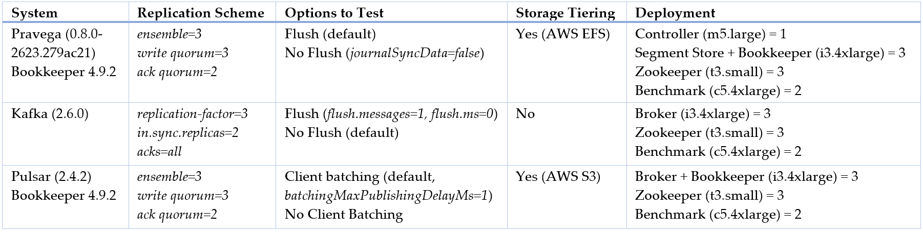
For all experiments, we use the same replication scheme of three replicas for each message or event and two acknowledgements required to complete a write. We configured Pravega to use an AWS EFS volume for LTS, and Pulsar to offload data to storage (AWS S3); for Kafka, this feature is not available in open source at the time of this writing. Note that configuration values other than the ones specified in this blog post have the defaults used in the official OpenMessaging Benchmark repo. All this information is summarized in the table below.

By default, our workloads use routing keys on writes (i.e., RANDOM_NANO key distribution mode in OpenMessaging Benchmark). We favor this option to ensure per-key event order, frequently a requirement of streaming applications for correctness. To be consistent with results in previous posts, we also execute workloads without routing keys to understand the potential impact of this decision (i.e., NO_KEY key distribution mode in OpenMessaging Benchmark).

To show the efficiency of the write path across all three systems, we perform the comparison using one drive to the BookKeeper journal for Pulsar and Pravega, and one drive to Kafka Broker log.

We plot latency and throughput for our results. In all graphs, the y-axis is in the logarithmic scale, while the x-axis is logarithmic or linear, depending on whether throughput refers to events or data, respectively. We want to keep the visual resolution on low and high throughput rates, which is not possible with the linear scale. The solid lines of plots refer to the default configuration of the systems (see table above), whereas the dotted lines refer to a specific configuration setting, described accordingly. We also provide tables with the plots that include the values plotted, other latency percentiles (i.e., 50th and 99th percentiles) and the raw benchmark output in all the experiments. Finally, note that the results plotted here are representative but subject to variability across executions, given the multi-tenant nature of AWS (for more info about expected variability, please read this section). Such variability is more prevalent in cloud environments than in on-premises, controlled ones.

Unbounded Pravega Streams

Ingesting and storing unbounded data streams enables an application to read and process both recent and historical data. From the perspective of the application, there are five relevant points when interacting against Pravega:

Data ingestion: As data sources generate data, Pravega must capture and store such data efficiently and in a durable manner.
Tailing a stream: Applications are often latency sensitive and Pravega must deliver data end-to-end with low latency and strict ordering guarantees.
Catching up: It is not unusual that a reader process for an application tailing one or more streams starts from scratch or is restarted. In such cases, the reader must be able to read with high throughput to catch up with the tail of streams eventually.
Historical processing: Even though stream processing typically refers to processing the tail of the stream, it is also desirable to process historical data as part of validation or further off-line processing for comprehensive insights.
Elasticity: As the ingest workload fluctuates, a stream automatically increases and decreases parallelism by scaling up and down, respectively, with auto-scaling.

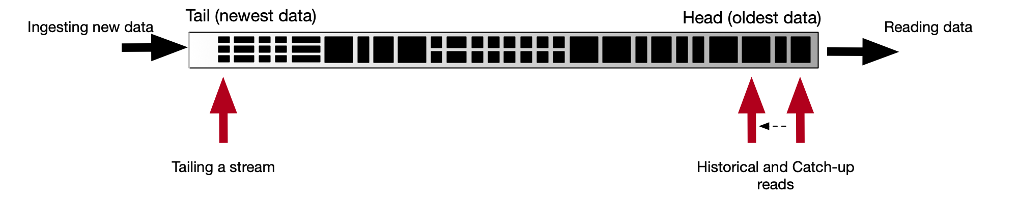
Figure: Ingesting, tailing, catching up, and reading historically from a Pravega stream.

In the following sections, we explore each one of these points from a performance perspective.

Ingesting stream data

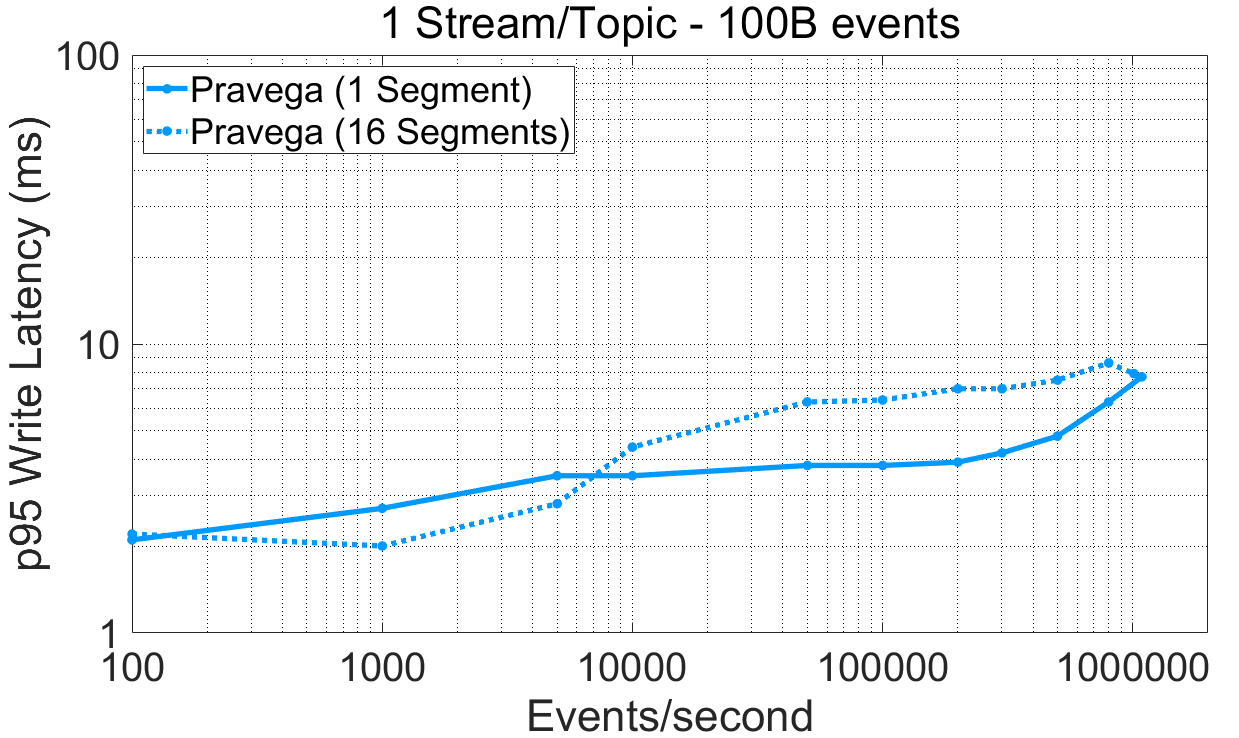
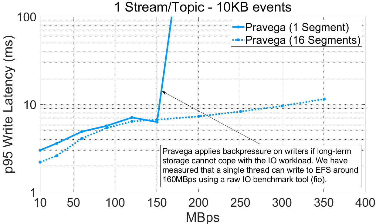
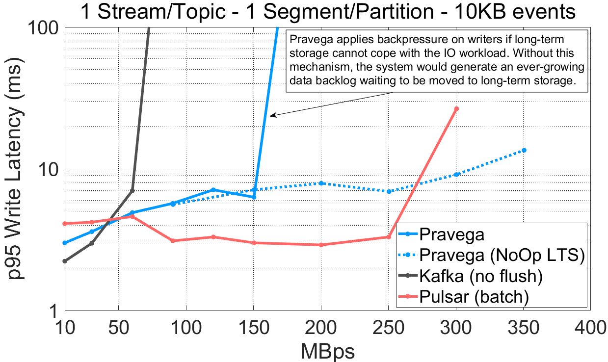
Low ingestion latency and high ingestion throughput. We initially analyze latency (plot 95th percentile) and throughput as a function of the ingestion rate for different event sizes and the number of segments used by the Pravega writer.

For Pravega, this experiment can be reproduced via P3 Test Driver using as input this workload file and this config file. The raw benchmark output is available here: 20-08-2020-pravega-080-randomkeys.

From the plots above, we highlight the following:

Irrespective of the event size and the number of segments, the Pravega writer achieves single-digit millisecond write latency (95th percentile) for various throughput rates.
A single Pravega writer can achieve around 1 million events per second for 100-byte events.
For small events (100 bytes), using multiple parallel segments in Pravega provides lower latency for low throughput rates while using one segment achieves lower latency for high throughput.
For large events (10K bytes), writing to multiple segments achieves higher throughput (350MBps) compared to a single segment (160MBps approx.). The throughput of a single segment is bottlenecked by the throughput of LTS, in this deployment, EFS. We have measured with fio the maximum write throughput to EFS for a single thread and obtained approximately 160MBps. Pravega, consequently, applies backpressure correctly once it reaches the throughput capacity of the LTS tier.

High throughput is important when ingesting data from arbitrary sources. It is equally relevant to deliver recent data with low latency for latency-sensitive applications. Imagine an Industrial IoT application with a large number of machines and a large number of sensors per machine continuously emitting data that need to be ingested and processed at the shortest time interval possible. Pravega satisfies both requirements when ingesting data across a wide range of event sizes. Also, Pravega applies backpressure to writers if long-term storage saturates, protecting the system from ever-growing backlogs.

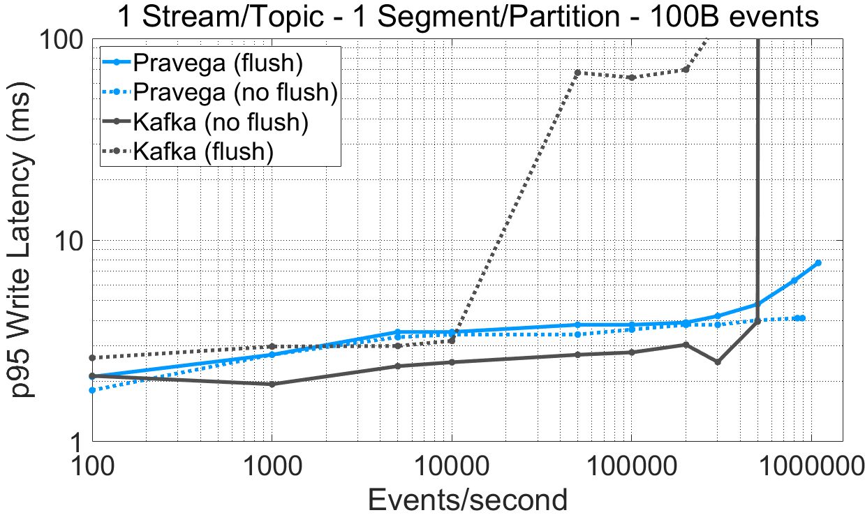
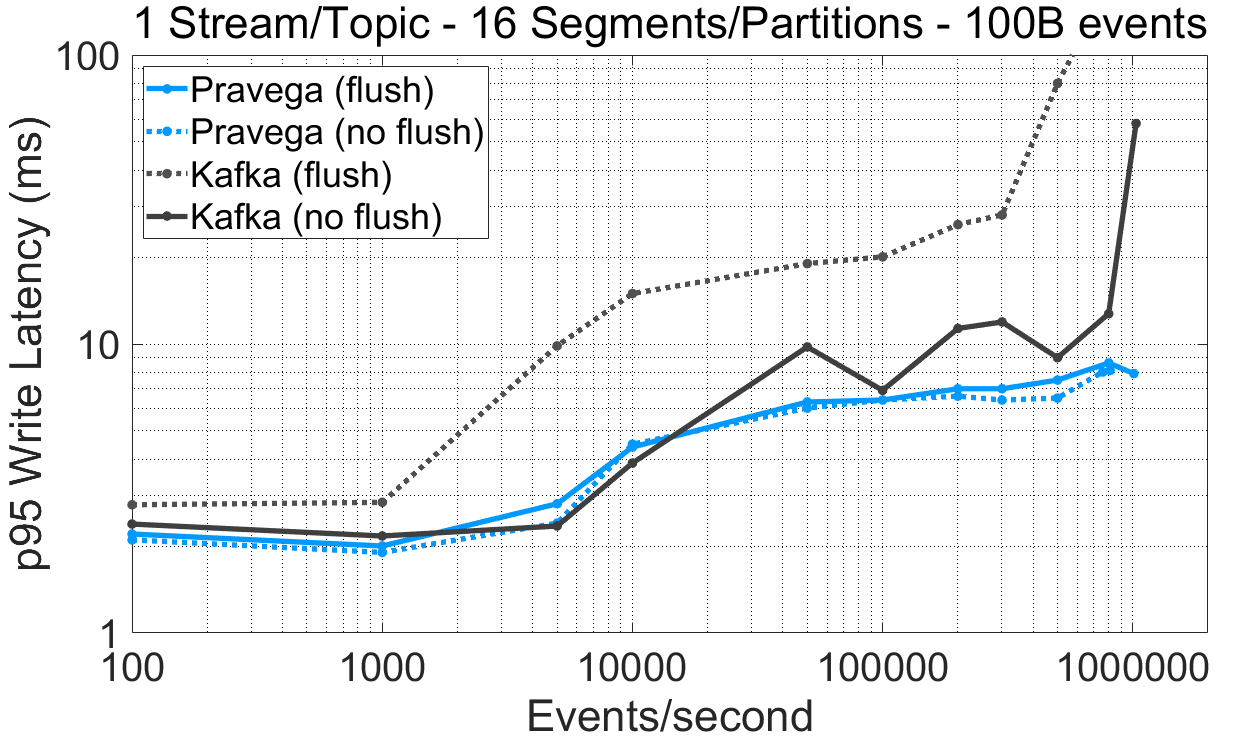
Durability upon ingestion. It is natural for an application to expect that data is available for reading once writing the data is acknowledged, despite failures. Durability is critical for applications to reason about correctness. Here, we show latency (95th percentile) and throughput to compare the performance implications of the different durability options. Specifically, we performed the following experiments:

A comparison of Pravega with and without durability; that is, enabling and disabling journal flushes in the durable log (Apache Bookkeeper, enabled by default).
A comparison with Apache Kafka with and without durability, a system that, by default, does not guarantee that data is on durable storage media upon acknowledgments.

Note that Kafka assumes that broker faults are independent and that the probability of correlated faults, such as all replicas stopping or crashing together, is negligible. This assumption is undesirable for any enterprise application as correlated failures do happen and servers do not always stop gracefully [3]. A wider swath of streaming applications are getting built for enterprises, and any enterprise-grade product needs to provide durability.

For Kafka, this experiment can be reproduced via P3 Test Driver using this workload file (varying durability) and this config file. The raw benchmark output is available here: 07-09-2020-kafka-260-confluent-randomkey-sync, 20-08-2020-pravega-080-randomkey-nosync, 04-09-2020-kafka-260-confluent-randomkey-nosync.

We draw the following observations from the experimental data:

For a stream/topic with one segment/partition, the Pravega writer (“flush”) reaches a maximum throughput 73% higher than Kafka (“no flush”). For 16-segments/partitions, the maximum throughput of both Pravega and Kafka is similar (over 1 million events/second).
Enforcing data durability for Kafka (“flush”) has a major performance impact on write latency. This is especially visible for moderate/high throughput rates. Kafka flushes messages according to a time (log.flush.interval.ms) or a message (log.flush.interval.messages) interval. When the message interval is set to 1, all messages are flushed individually before being acknowledged, inducing a significant performance penalty. With Bookkeeper, data is persisted before being acknowledged, but they are opportunistically grouped upon flushes [4].
The latency benefit for Pravega of not flushing data to persistent media for Bookkeeper writes is modest, which justifies providing durability by default.
For latency and a stream/topic with 1 segment/partition, Kafka (“no flush”) gets consistently lower (~1ms at p95) write latency than Pravega (“flush”) up to 500K e/s. For all the other cases, Pravega producer shows lower latency than Kafka (“no flush”).

The default Kafka producer (“no flush”) achieves similar write latency and lower throughput compared to the Pravega (“flush”) producer (less than 1ms difference) up to the point in which it saturates, while sacrificing data durability. When Kafka ensures data durability (“flush”), performance degrades, both saturating earlier and presenting higher latency, and impacting especially the case with 16 segments.

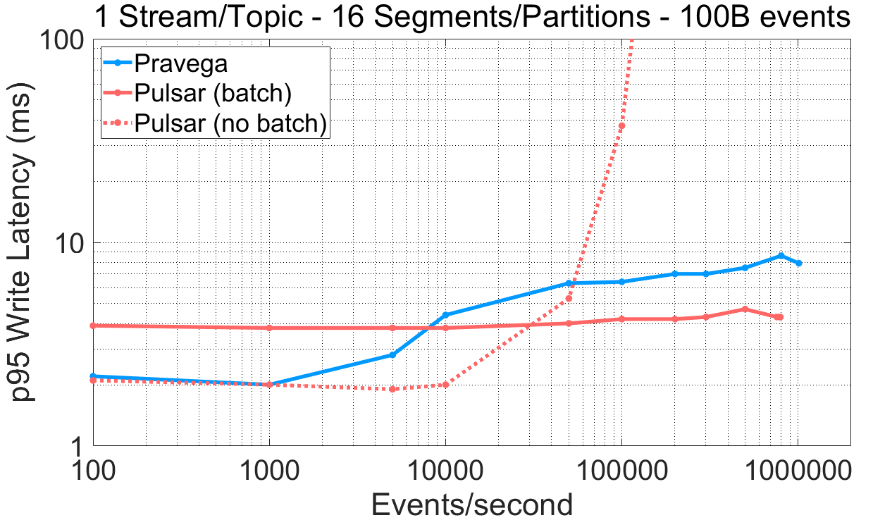
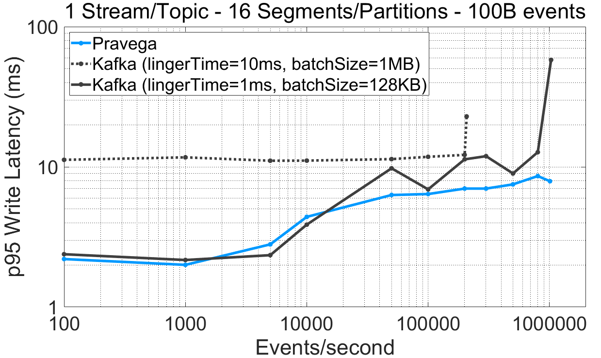
Dynamic client batching vs. knobs. Batching enables a trade-off between throughput and latency. Applications ideally do not need to reason about convoluted parameters to be able to benefit from batching, and it should be the work of the client library along with the server to figure it out. This goal is precisely the one of a dynamic batching heuristic that Pravega introduced in the writer.

Here, we plot latency (95th percentile) and throughput to understand the impact of Pravega writer batching on performance. We contrast Pravega against Apache Pulsar and Apache Kafka (“no flush” by default), which are systems that require an application to choose between whether to use batching or not, and configure it accordingly.

For Pulsar, this experiment can be reproduced via P3 Test Driver using as input this workload file (varying the batching flag) and this config file. The raw benchmark output is available here: 10-09-2020-pulsar-242-tiering-randomkey-nobatch, 09-09-2020-pulsar-242-tiering-randomkey-batch, 07-09-2020-kafka-260-confluent-randomkey-nosync-largebatch.

Based on the previous results, we highlight the following:

The Pulsar producer is designed to target either low latency or high throughput, but not both. This forces the user to choose between a latency-oriented (“no batch”) or a throughput-oriented configuration (“batch”).
Pravega achieves both lower write latency than Pulsar (“batch”) for the lower-end of throughput rates (e.g., <10K e/s) and higher maximum throughput than Pulsar (“no batch”).
Increasing the batch size and the linger time for Kafka (10ms linger time, 1MB batch size) to enable more batching has the opposite expected effect. The throughput drops compared to a configuration with 1ms linger time and 128KB batch size. To understand this result, we inspected the maximum throughput of a Kafka producer writing to a 16-partition topic and using the same batch configuration, but without using routing keys when writing data (NO_KEY option in the OpenMessaging Benchmark). In this case, the client achieved 120MBps instead of 20MBps. We consequently attribute the lower performance we observed to selecting routing key randomly.

Dynamic batching in Pravega allows writers to achieve a reasonable compromise between latency and throughput: it obtains single-digit millisecond latency for low and high throughput rates, while smoothly trading latency for throughput as the ingestion rates increase. Pravega does not require the user to decide the performance configuration of the writer ahead of time, and the use of routing keys does not impact its mechanism.

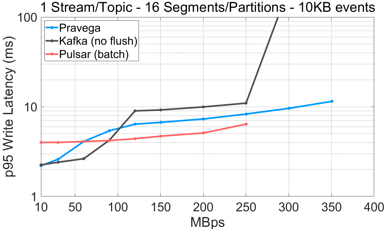
Large events and high byte-throughput rates. Events are often small in real applications, say 1Kbyte or less, but there is no shortage of use cases with larger events. For such scenarios, batching is less effective, and the most relevant metric is the byte rate with which we can ingest. For this part of the experiments, we use 10Kbyte events, and we compare it with both Pulsar and Kafka. We plot latency (95th percentile) and throughput, but we use byte-throughput rather than event-throughput on the x-axis.

The data for this experiment is built upon the previous experiments (workload and config files).

Inspecting the previous results, we observe that:

- For a single-segment/partition stream/topic, Pravega (160MBps) and Pulsar (300MBps) writers achieve a much higher write throughput compared to Kafka (70MBps).
- For a 16-segment/partition stream/topic, Pravega achieves the highest throughput (350MBps) compared to Kafka (330MBps) and Pulsar (250MBps).
- Visibly, Pravega cannot write faster than 160MBps in the single-segment case; it is again bottlenecked by EFS. To validate that Pravega EFS indeed bottlenecks Pravega, we have conducted an experiment using a test feature that makes Pravega write only metadata to the long-term storage tier and no data (“NoOp LTS“). From the results, skipping the data writes to LTS enables much higher throughput for Pravega (350MBps).
- Pulsar performs better with tiering enabled for the single-segment case because it does not throttle when tiered storage is saturated. This problem becomes evident when we present historical read results further down.

Compared to Pulsar and Kafka, Pravega achieves high data write throughput when using multiple segments. The throughput of Pravega depends on the throughput capacity of LTS, and in the case LTS saturates, Pravega applies backpressure to avoid building a backlog of data. LTS is an integral part of the Pravega architecture, and Pravega adjusts overall system performance according to LTS.

Tail Reads

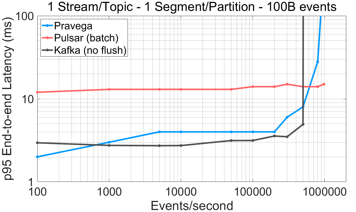
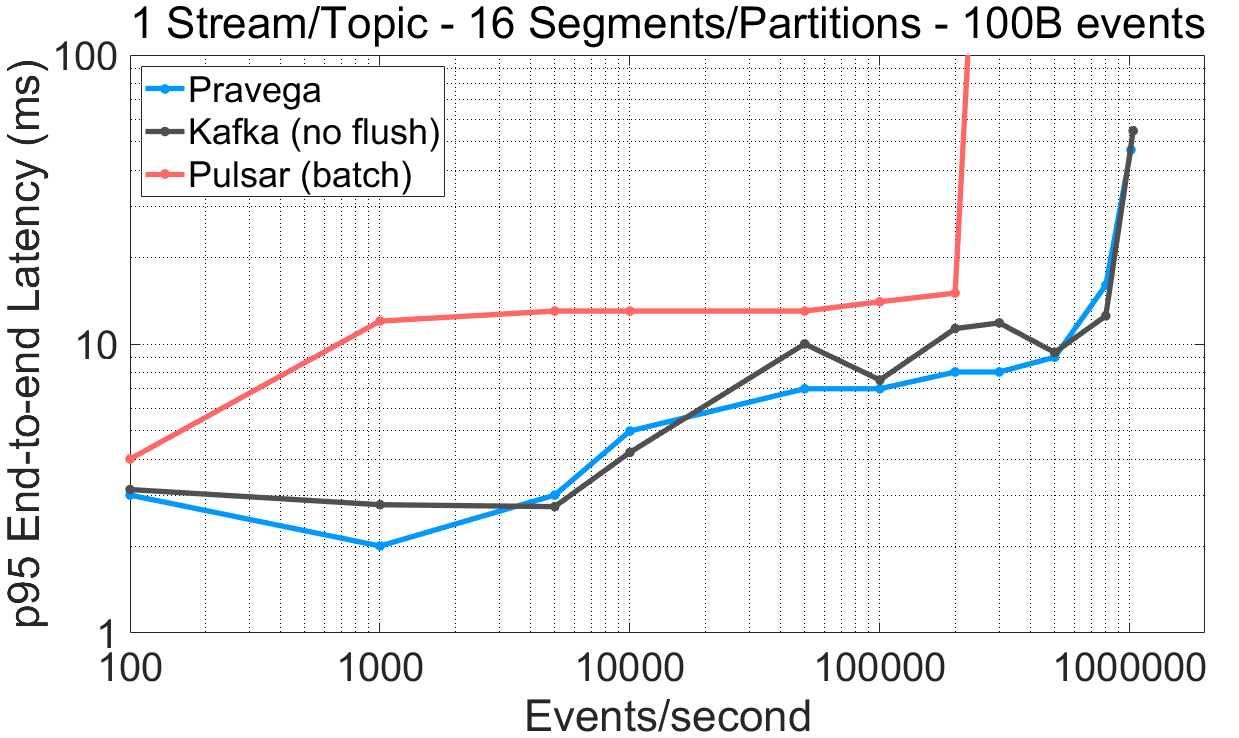
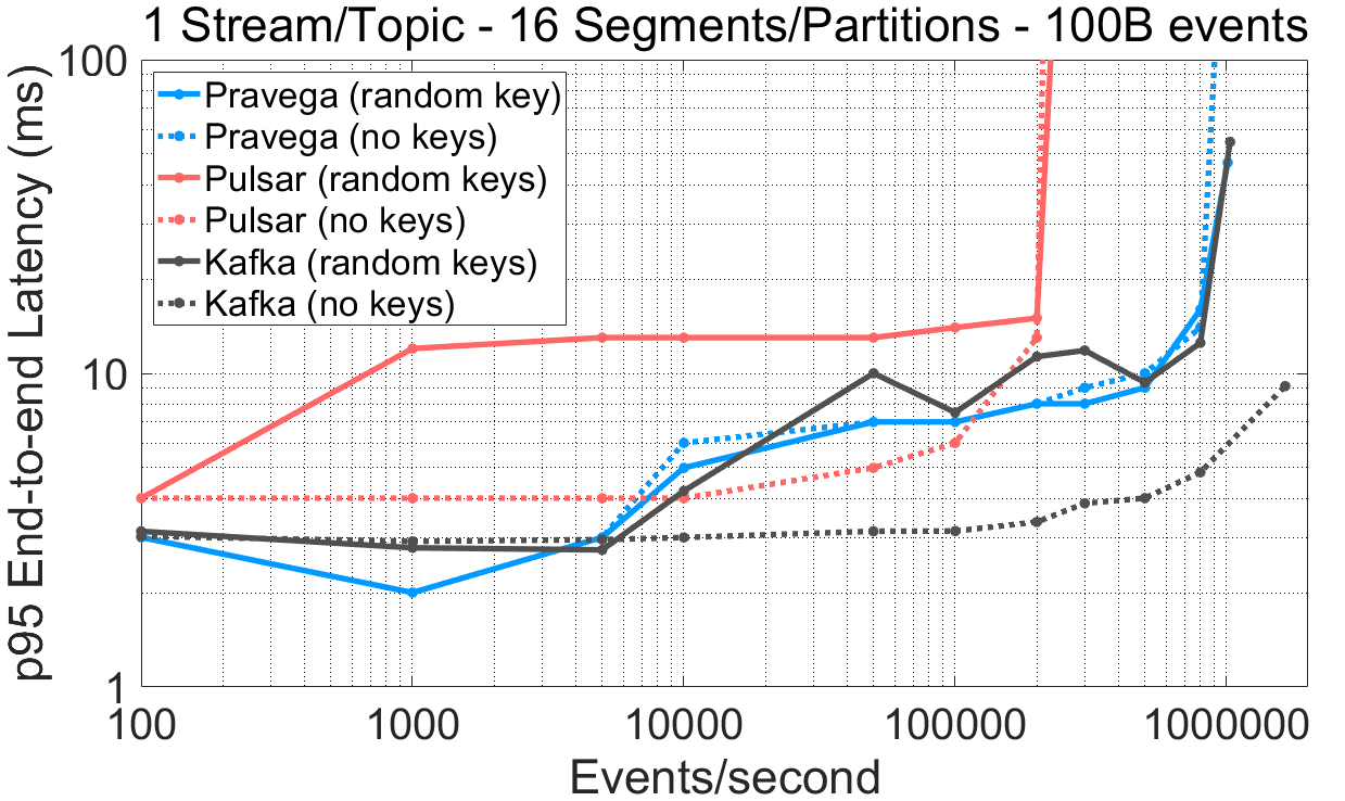
Low-latency, parallel reads. For many applications, the time must be short between the event being generated and the time that it is available for reading and processing. We refer to such a time interval as end-to-end latency. The streaming cache, a homebrewed cache the Segment Store uses, plays a key role in the end-to-end latency. We plot the end-to-end latency and throughput for 100B events, contrasting the performance with both Pulsar and Kafka.

The data for this experiment is built upon the previous experiments (workload and config files).

We highlight the following from these experiments:

For a stream/topic with a single segment/partition, Pravega and Kafka exhibit lower end-to-end latency compared to Pulsar up to the saturation point. Pulsar does not achieve end-to-end latency values under 12ms (95th percentile), even with batching.
Read throughput for a stream/topic with a single segment/partition is much higher for Pravega (72%) and Pulsar (56%) than Kafka.
Interestingly, for a stream/topic with 16 segments/partitions, Pulsar shows a 76% drop in read throughput than the single segment/partition case, despite configuring one consumer thread per segment/partition in all systems (higher read parallelism). In the case of Kafka, managing more segments increases end-to-end latency.
For 16 segments/partitions, the Pravega reader achieves similar or better end-to-end latency numbers than Kafka. Note that the Pravega Streaming Cache serves both tail readers and asynchronous writes to LTS concurrently, whereas Kafka does not perform any storage tiering task.

Pravega provides low end-to-end latency compared to Kafka and Pulsar, thus satisfying the requirements of latency-sensitive applications that need to tail ingested stream data.

Guaranteeing order for readers. Per-key event ordering is desirable for a number of applications to enable correct processing of the events while providing parallelism. All of Pravega, Pulsar and Kafka use routing keys and guarantee total order per key.

Next, we compare the read performance of Pravega, Pulsar (“batch”) and Kafka (“no flush”) when OpenMessaging Benchmark is instructed to not use routing keys (NO_KEY) vs. when random keys from an existing set are used (RANDOM_NANO, used in all the experiments by default).

This experiment is the same as previous ones but using NO_KEY instead of RANDOM_NANO as routing key scheme in OpenMessaging Benchmark. The raw benchmark output is available here: 07-09-2020-kafka-260-confluent-nokey-nosync, 09-09-2020-pulsar-242-tiering-nokey-batch, 20-08-2020-pravega-080-nokey.

The results above reveal differences in the performance of other systems concerning the presence of routing keys:

Using multiple routing keys across several topic partitions induces a significant read latency overhead in Pulsar compared to not using routing keys. This phenomenon is visible for both small and large events.
For 100B events, when Kafka does not guarantee order (NO_KEY) or durability (“no flush”), read (and write) performance is higher, both latency and throughput, for 16 segments.
According to the documentation of Pulsar and Kafka, these clients exploit client-side batching when no routing keys are used as they distribute load across partitions (round-robin fashion) based on batches, not events. This decision also seems to impact the performance of readers.
Pravega is not significantly impacted if an application requires multiple routing keys across segments to guarantee order, making its performance consistent across applications and use cases.

Kafka, Pulsar and Pravega guarantee strict event ordering based on routing keys. However, a workload interleaving multiple routing keys when writing events in Pulsar and Kafka performs worse than when using no routing keys. This observation is particularly evident in the case of multiple parallel segments/partitions. In contrast, Pravega’s performance is consistent irrespective of the use of routing keys. As many applications use routing keys for ordering, it is crucial to highlight the performance difference that using no routing key induces compared to keys with different access distributions (e.g., uniformly distributed, heavy-tailed, strict subset, etc.). We do not claim that RANDOM_NANO is an option representative of several realistic scenarios, but it indeed shows a deficiency when using the NO_KEY option to evaluate performance and stresses systems further.

Historical and Catch-Up Reads

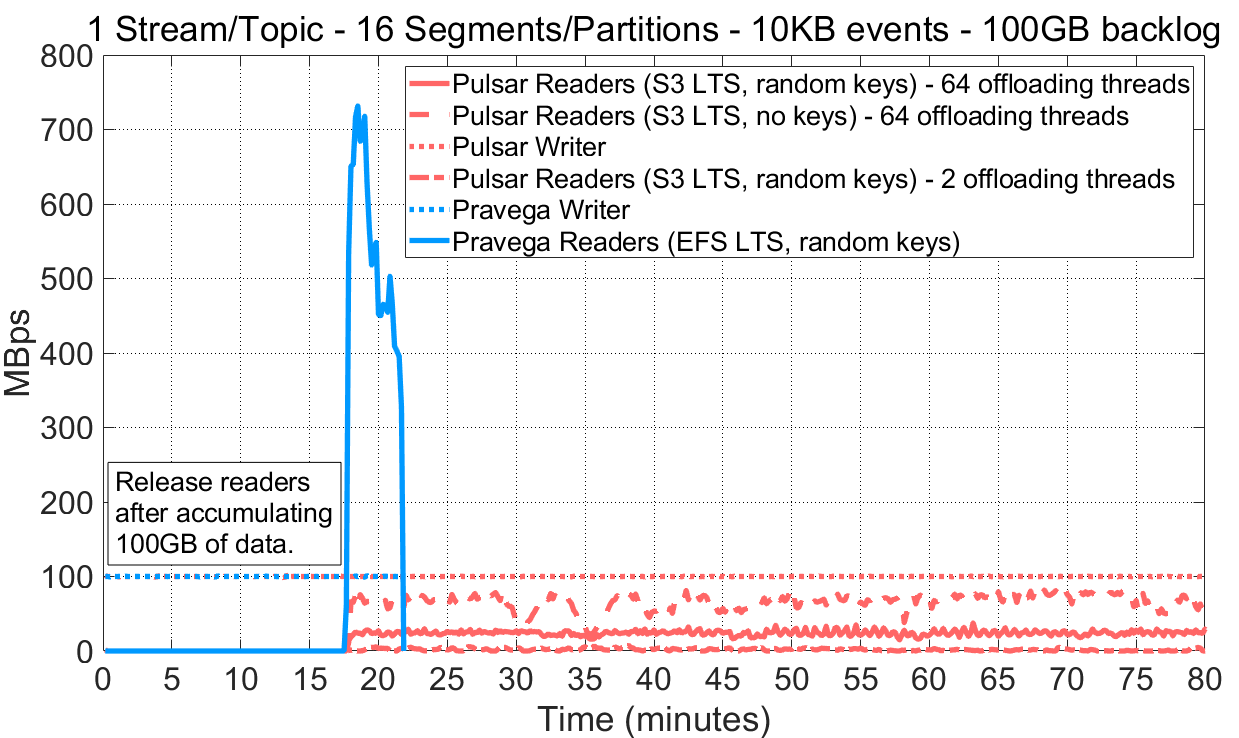
In this set of experiments, we analyze the performance of readers when requesting historical data from long term storage in Pravega and Pulsar (at the time of this writing, Kafka does not provide this functionality in open source). We designed the experiment as follows.

OpenMessaging Benchmark has an option called consumerBacklogSizeGB that essentially holds readers until writers have written the amount of data specified. Readers are subsequently released, and the experiment completes when the backlog of messages is consumed. We exercised this option by configuring writers to write 100MBps (10KB events) to a 16-partition/segment topic/stream at a constant rate until achieving a backlog of 100GB. Note that writers continue to write data when readers are released, so readers should read faster that the write throughput to catch up.

This experiment can be reproduced via P3 Test Driver using as input these workload files for Pulsar and Pravega. The raw benchmark output is available here: 13-08-2020-pulsar-nokey-tiering-64threads-historical, 13-08-2020-pulsar-randomkey-tiering-64threads-historical, 17-08-2020-pulsar-randomkeys-tiering-2threads-historical, 19-08-2020-pravega-080-randomkey-historical.

Looking at how readers behave reading from long term storage, we highlight the following:

Pravega achieves much higher read throughput from long-term storage compared to Pulsar. For Pulsar, we have tried different tiering configuration parameters (e.g., ledger rollover) with similar results. Also, we have compared the throughput of EFS and S3. We obtained close throughput rates for individual file/object transfers (i.e., 160MBps approx.); this implies that such an important difference in historical read performance between both systems is not due to long-term storage.
Pravega can throttle writers in case that long-term storage cannot absorb the ingestion throughput. Pulsar does not implement this mechanism, which leads to situations of imbalance across storage tiers. As shown in the results above, writers are faster than readers reading from long term storage, so the backlog of messages to be read grows without bounds.
Visibly, aspects like the number of offloading threads or the routing keys used in Pulsar have a significant impact on the performance of historical reads. However, there is no clear set of guidelines for users to configure tiered storage.

Both Pravega and Pulsar provide means to move historical data to a long-term storage tier. Pravega achieves much higher historical read throughput compared to Pulsar and offers IO control of data across tiers, thus preventing ingestion backlogs from building. Pravega achieves it transparently without user intervention or complicated configuration settings. As mentioned before, we have not had access to an open-source version of Kafka to compare against.

Pravega Autoscaling: Making streams elastic

Accommodating workload fluctuations over time through stream auto-scaling is a unique feature of Pravega. The absence of this feature in systems like Pulsar and Kafka, which are primarily on the front-line of big data ingestion, induces considerable operational pain to users, particularly at scale.

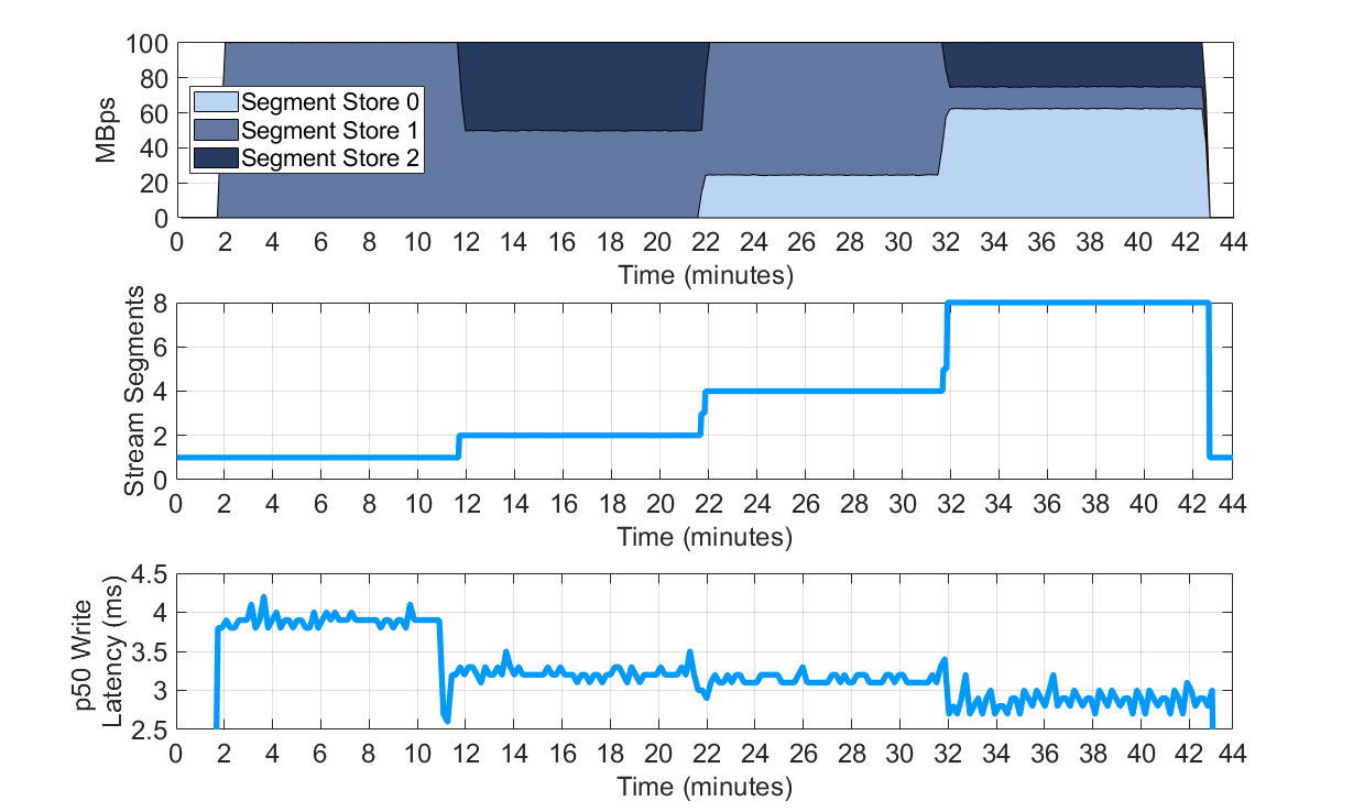
We focus in this section on the performance implications of stream auto-scaling. We enabled in the OpenMessaging Benchmark Pravega driver configuration the auto-scaling flag (enableStreamAutoScaling). We set the target rate of events per second on Segments to 2,000 (or 20MBps, as in this experiment we have used 10KB events). The benchmark tool wrote at a speed of 100MBps. Note that to generate some of the plots below we have used the Pravega metrics exported to InfluxDB and Grafana (deployed on each experiment for analysis purposes).

The three plots show different aspects of stream auto-scaling in Pravega: i) the write workload per Segment Store, ii) the number of segments in the stream, and iii) the write latency perceived by the OpenMessaging Benchmark instance.

This experiment can be reproduced via P3 Test Driver using as input this workload file for Pravega and this config file. The raw benchmark output is available here: 19-08-2020-pravega-080-randomkey-autoscaling.

These are the main points we highlight from this experiment:

At the time of this writing, Pravega is the only system providing dynamic and transparent repartition of a stream based on target rates while preserving the order of segments. In systems like Pulsar or Kafka, repartitioning a topic requires manual intervention.
As the Pravega stream splits and adds more segments, the load is distributed across the available segment stores and causes latency to drop.
The distribution of segments in Pravega is stateless and based on consistent hashing.

The precise distribution of stream load across the system depends on the number of segment stores available and segment containers configured. Landing multiple segments on the same segment container provides additional capacity to the stream if the segment container has spare capacity. Adding more segment containers to a deployment increases parallelism as segment containers write to independent durable logs, and increases the chances that two segments of a stream upon scaling do not end in the same segment container. A larger number of segments also increases the probability of an even distribution of load across segment stores and containers.

Pravega is the first storage system that provides elastic streams: data streams that are automatically repartitioned according to ingest load. Auto-scaling improves performance when load demands are high by utilizing resources across the cluster more efficiently. Applications enable auto-scaling via stream configuration, requiring no other intervention during execution.

Wrap Up

Streaming data requires both low latency and high throughput; Pravega is able to provide both simultaneously. A single Pravega writer is able to sustain over 1 million events per second with a p95 latency under 10ms. It adapts batching according to the ingestion workload, avoiding users to choose ahead of time between high throughput or low latency for their applications. Tiering stream data to LTS is an integral part of the Pravega architecture, necessary for historical processing. Pravega enables readers to catch up with large backlogs while writers are adding 100s of megabytes per second, while ensuring that LTS can sustain the ingestion rate. These performance traits of Pravega hold both when using routing keys for ordering and when omitting them.

When contrasting Pravega results with other systems, Kafka and Pulsar, we realized that both systems present an important performance difference between using routing keys to publish messages and omitting them. For both systems, the latency doubles when using routing keys and, specifically for Kafka, the read throughput is about 1/3 lower.

Foregoing durability in Kafka is not necessarily effective as it presents similar/lower throughput and higher latency compared to Pravega, and Pravega always guarantees durability. Pulsar makes applications choose between low latency and high throughput, and provides lower end-to-end performance with more topic partitions.

Features like tiered storage and scaling are effective in handling historical processing and providing stream elasticity. Pravega was the first system among the three to provide tiered storage, and others followed. We tested Pulsar implementation of tiered storage and were not able to obtain a reasonable throughput, inducing the formation of a backlog. Stream scaling is still a feature that is unique to Pravega.

Even though we have covered quite a bit of ground in this post, performance evaluation is not a bounded task; there are different dimensions to cover and the performance of systems evolve with code changes. We focused here on basic read/write functionality, which we believe is a fundamental first step. Pravega is inherently built as a cloud-native, scale-out system and we expect Pravega to shine when we talk about scalability and other aspects, so stay tuned for new posts from us.

Acknowledgments

This blog post is the result of team effort for various months. From all the people involved, we especially thank Andrei Paduroiu and Tom Kaitchuck for their continuous effort with the analysis and the performance improvements, and Srikanth Satya for guiding us throughout this exercise with immense technical wisdom. We acknowledge Pavel Lipsky, Maria Fedorova and Tim Butler for numerous early and late hours investigating the performance of Pravega that led to the results here. We thank Ashish Batwara for the countless hours helping us to orchestrate the work and for providing the necessary resources to realize this post, and Igor Medvedev for helping us to shape it.

About the Authors

Raúl Gracia is a Principal Engineer at DellEMC and part of the Pravega development team. He holds a M.Sc. in Computer Engineering and Security (2011) and a Ph.D. in Computer Engineering (2015) from Universitat Rovira i Virgili (Tarragona, Spain). During his PhD, Raúl has been an intern at IBM Research (Haifa, Israel) and Tel-Aviv University. Raúl is a researcher interested in distributed systems, cloud storage, data analytics and software engineering, with more than 20 papers published in international conferences and journals.

Flavio Junqueira is a Senior Distinguished Engineer at Dell. He holds a PhD in computer science from the University of California, San Diego, and he is interested in various aspects of distributed systems, including distributed algorithms, concurrency, and scalability. His recent work at Dell focuses on stream analytics, and specifically, on the development of Pravega. Before Dell, Flavio held an engineering position with Confluent and research positions with Yahoo! Research and Microsoft Research. Flavio has co-authored a number of scientific publications (over 4,000 citations according to Google Scholar) and an O’Reilly ZooKeeper book on Apache ZooKeeper. Flavio is an Apache Member and has contributed to projects hosted by the ASF, including Apache ZooKeeper (as PMC and committer), Apache BookKeeper (as PMC and committer), and Apache Kafka.

References

[1] John Paulsen. “Enormous Growth in Data is Coming — How to Prepare for It, and Prosper From It”, April 2017.
[2] Stephanie Condon. “By 2025, nearly 30 percent of data generated will be real-time, IDC says“, Nov. 2018
[3] Yigitbasi, Nezih, et al. “Analysis and modeling of time-correlated failures in large-scale distributed systems.” 2010 11th IEEE/ACM International Conference on Grid Computing. IEEE, 2010.
[4] Junqueira, Flavio P., Ivan Kelly, and Benjamin Reed. “Durability with bookkeeper.” ACM SIGOPS Operating Systems Review 47.1 (2013): 9-15.
[5] Gracia-Tinedo, Raúl, et al. “SDGen: Mimicking datasets for content generation in storage benchmarks.” 13th USENIX Conference on File and Storage Technologies (FAST’15). 2015.
[6] Iosup, Alexandru, Nezih Yigitbasi, and Dick Epema. “On the performance variability of production cloud services.” 2011 11th IEEE/ACM International Symposium on Cluster, Cloud and Grid Computing. IEEE, 2011.

Appendix

Only read this if you know what you are doing — The gory details of our experimental setup

In this section, we describe in detail how we have deployed Pravega on AWS as well as the technical configuration details of the environment. For comparison and reproducibility, we have based our investigation on the two blog posts we mentioned previously.

Benchmark setup on AWS. We executed our experiments with OpenMessaging Benchmark, an open and extensible benchmark framework for messaging. The exact code we have used to carry out the benchmarks is in this repository, and concretely, using this release. The main reason for using our own fork of OpenMessaging Benchmark is to make available the Pravega driver while it in process of being accepted by the community. Apart from that, we have also added minor changes to Pulsar in our fork to elaborate this blog post (e.g., tiering configuration for Pulsar topics), as well as minor bug fixes that will be submitted progressively as contributions to mainline. For Kafka, we use the OpenMessaging Benchmark driver recently published in this repository (commit id 6d9e0f0) by Confluent, as authors claim that it fixes several performance problems. To quickly use the new Kafka driver in our methodology, we recommend to git apply this patch (i.e., it keeps reporting format consistent with our OpenMessaging Benchmark fork, fixes drives names for our instances, allows to execute P3 driver, etc.).

The exact deployment instructions for Kafka and Pulsar can be found in the official documentation page. For brevity, we have detailed the exact steps to deploy Pravega in the documentation of the driver; it is a very similar process compared to its counterparts. While all the deployment details are in the documentation, it is worth noting that it is necessary to fulfill some pre-requisites to be able to experiment on AWS, including having access to an AWS account, installing and configuring the AWS CLI, and setting up the appropriate SSH keys.

For the sake of fairness, another important aspect to consider is to use same type of EC2 instances for deploying the analogous components of each system. In their respective Terraform files, you can observe the instance types used to deploy Pravega, Kafka and Pulsar. It is especially relevant to mention that for the components in charge of writing data (i.e., Broker, Bookkeeper), we use an instance type with access to local NVMe drives (i3.4xlarge). In our experience, using local drives allows us to push the systems to their limit, which is what we look for in a performance evaluation. As this blog post mainly evaluates the write and (tail) read paths of systems, we provide the same amount of drives relevant to the critical write path (1 drive for Bookkeeper journal in Pravega and Pulsar, 1 drive to Kafka log).

Configuration of systems. One of the key configuration aspects for a performance evaluation of storage systems is replication. Data replication is widely used in production environments, as it provides data availability at the cost of extra overhead related to generate redundant data. While the replication schemes differ between Apache Kafka (leader-follower model) and Pravega/Pulsar (Bookkeeper uses a quorum-vote model), we can configure them to achieve a similar data redundancy layout. We configured all the systems to create three replicas of every message, requiring at least two of such replicas to be confirmed by the servers before considering a write as successful.

Interestingly, there is an important difference between the default behavior of Kafka versus Pravega/Pulsar in terms of data durability. For context, calling write() on the file system is not enough to have the data durably stored in persistent storage. As a well-known performance optimization technique, modern file systems use a special memory region called “page cache” to buffer small writes, which are moved asynchronously to disk based on the OS decision. But, given that the page cache is not persistent, the ultimate consequence is that data can be lost if upon a crash there is data not yet written to disk. To prevent that from happening, any application should explicitly flush writes (fsync system call) to ensure that data is persisted on disk. That said, Kafka by default does not flush data, thus trading-off durability in favor of performance. In this sense, we want to evaluate what is the actual price that Kafka pays to achieve the same durability guarantees as Pravega and Pulsar by default (i.e., by setting flush.messages=1, flush.ms=0).

For memory, we need to distinguish between the benchmark workers and the server-side instances of the systems under evaluation. To keep benchmark worker instances consistent with Confluent’s blog post, we use 16GB as JVM heap space in all our experiments. At the server side, Kafka memory settings are detailed here. Bookkeeper (version 4.9.2) settings are the same for Pulsar and Pravega (6GB of JVM and 6GB of direct memory). For Pulsar brokers, we defined 6GB of JVM heap and 6GB of direct memory as well. Similarly, in Pravega we also defined 6GB of JVM heap memory and 20GB of direct memory, given that Pravega implements an in-memory cache that is set to 16GB and utilizes direct memory (the cache is the only place where client reads are performed in Pravega).

It is important to note that Pravega is inherently moving ingested data to long-term storage (LTS). In our experiments, we used an NFS volume as backed up by an AWS Elastic File Service (EFS) instance (provisioned with 1000MBps of throughput). For fairness, we also have enabled tiering in Pulsar to compare against Pravega when both systems are carrying out the same tasks. We have configured for Pulsar an AWS S3 bucket and defined the ledger rollover to happen within 1 and 5 minutes, so tiering activity occurs while benchmark take place (managedLedgerMinLedgerRolloverTimeMinutes=1, managedLedgerMaxLedgerRolloverTimeMinutes=5, managedLedgerOffloadMaxThreads=[2|64 (default)]). We also set Pulsar topics within the benchmark namespace to start the offloadding process immediately (setOffloadThreshold=0), as well as to remove the data from Bookkeeper as soon as it is migrated to long term storage (setOffloadDeleteLag=0). Unfortunately, at the time of this writing Kafka does not provide tiering in its open source edition (only recently, in its enterprise edition).

Client configuration. Pulsar and Kafka clients implement a batching mechanism that can be parameterized via “knobs”, also in the context of OpenMessaging Benchmark experiments. This feature enables the Pulsar producer to buffer a certain number of messages (batchingMaxMessages or batchingMaxBytes) or wait until some timeout (batchingMaxPublishDelayMs) before performing the actual write against the Broker. Similarly, in Kafka we find the analogous parameters, namely, batch.size and linger.ms. The goal of this feature is to improve a producer’s throughput for small messages, despite inducing extra latency in scenarios where the workload is not throughput-oriented. By default, we use in both systems a similar configuration: 128KB as batch size and 1ms as batch time. We also compare the behavior of the Pulsar producer with and without this feature, as well as the impact of larger batches in Kafka (1MB as batch size and 10ms as batch time). Apart from that, the Pulsar client offers to enable data reduction techniques, such as compression. As such techniques may have a significant impact on performance depending on the data at hand, we did not enable them [5].

Workloads. In this post, we are interested in understanding the behavior of these systems based on two parameters: event size and number of partitions/segments. While there are many other interesting aspects to explore, these two are, perhaps, the first ones that an application developer may think about. Regarding the former, we consider small events (100B) and large events (10KB). The payloads used are the ones included in the official repository. Note that there are use-cases that could justify events to be much larger (e.g., media streaming), but the proposed ones can be considered as representative sizes for many typical streaming applications (e.g., logs, IoT, social media posts, etc.). For the latter parameter, we consider the streams/topics with 1 and 16 segments/partitions, so we can evaluate the impact of parallelism on the performance of client applications. Note that for 16 segments/partitions experiments, we configured 16 consumers (threads) on the reader VM to exercise the compute parallelism of readers (there is always only 1 writer in the writer VM irrespective of the segments/partitions).

An important point of the workload is related to the use of routing keys, which is the mechanism that most streaming systems use to provide the notion of event order. As ordering is a standard requirement in today’s streaming applications, we use by default in all our experiments one of the available routing key distributions in OpenMessaging Benchmark (RANDOM_NANO), which picks routing keys at random on each event write from a set of keys generated in advance (10K keys by default). We also want to compare if the use of routing keys has any impact on the systems under evaluation, so we also executed workloads without routing keys (NO_KEY mode in OpenMessaging Benchmark) to evaluate this specific aspect.

All the tests we started with a warm-up phase (1 minute) before the actual benchmark in which we gathered metrics. The workloads we used consist of writing and reading at a constant rate, whereas the benchmark continuously outputs latency and throughput values (4 minutes). Such values are the ones we use to generate our plots and result tables. Besides, the deployment scripts of these systems also include services to collect and expose metrics (e.g., Prometheus, InfluxDB), which we also use to give additional insights in some of the experiments.

While our workloads are based on the original ones on the OpenMessaging Benchmark repository (defined as YAML files), we noticed that just using the workloads available could be unnecessarily limited. For this reason, we automated the generation of latency vs throughput plots for all these systems via the P3 Test Driver. Essentially, this tool helps us to orchestrate the execution of benchmarks (e.g., changing the producerRate field in the official workloads), as well as to collect the metrics and generate the plots. With these latency-throughput plots, we can have a broader understanding of the behavior of these systems in a variety of scenarios.

Metrics. This post focuses on throughput as well as on two latency metrics, namely write latency and end-to-end latency. Throughput represents the amount of data, measured in events or byes per second, that a producer/consumer can write/read to/from the system. Note that in most tests will set the throughput as a constant to observe the behavior of latency.

On the one hand, write latency represents the time taken for the benchmark tool since an event is submitted for writing until the event is acknowledged back from the server. As writes are asynchronous, there is a callback on messages to calculate this metric once the response from the server arrives. Note that this metric is calculated on a single VM, and therefore there are no clock-related issues. On the other hand, end-to-end latency is the time elapsed since a writer writes an event up to the reader reads it. To get this metric, the payload of an event contains a timestamp representing the moment at which it was written. On the reader side, the metric is calculated as the delta between the timestamp in the payload and the current time. Given that writers and readers run on separate VMs to avoid interferences, we need to ensure that clocks do not differ (significantly) between them. To keep clocks in sync, client VMs executing OpenMessaging Benchmark run Chrony plus AWS Time Sync Service.

Performance variability observed in AWS. We observed some degree of performance variability when executing experiments on AWS. Such variability is expected due to the dynamics of a multi-tenant cloud [6]. We wanted to understand how such variability affects the numbers we produced, and quantified it with our experiments across several weeks. A sample of executions we have performed can be seen in the table below by picking two points: a low throughput point and a high throughput point. The results are in the table below:

Visibly, the most impacted metric is the maximum throughput of small events that a writer can achieve. For instance, from the Pravega runs captured in the table above, we see that the results with the highest event throughput is 14% higher (1.088M e/s) compared to the run to the lowest throughput (0.9532M e/s). As the maximum throughput of small events is basically a CPU intensive task at the benchmark VM, it seems to be specially sensitive to concurrent workloads consuming CPU within the same cluster. On the other hand, we observe that latency for low throughput rates (i.e., 1000 e/s in table) is a more stable metric, specially for percentiles lower than 99th. Similarly, we also verified that high data throughput experiments are stable, meaning that IO is not as variable compared to the CPU of instances.